Using Sinkhorn divergence to measure image similarity

To quantitatively evaluate the difference between images, one often uses the mean square error (MSE). However, MSE is often too sensitive to local pixel values and ignores the global (in)variabilities of image content.

One example where MSE causes trouble is in template matching, where the goal is to align an image with its translated version. To nudge the misaligned image toward the correct location, we want to use a metric that gives a small value when the translation distance is small, and conversely, a large value when the distance is large. However, this is often not the case if we use MSE as a metric. The MSE score betwee two images will be significant, even if the translation between them is small. This is because the MSE approach average error across pixels, and a tiny translation can cause large differences in pixel values.

Are there image metrics that can capture global variabilities of images? I recently learned from Adler et al. (2017), Dukler et al. (2019), and Kothari et al. (2020) that one approach is to use the Sinkhorn divergence. In this approach, we treat images—after a proper normalization—as histograms; we then compare the distance between two histograms through optimal transport. Specifically, the entropy-regularized Wasserstein metric between two histograms \(a\) and \(b\) is defined as

where \(C\) is a cost matrix, and \(U(a, b) := \{T \in \mathbb{R}^{m \times n}_{+} : T 1_n = a, T^\top 1_m = b\}\) is the transportation polytope. The cost matrix stores all pairwise costs between points in the supports of the histograms. That is, \([C]_{ij} = c(x_i, x_j)\) with \(x_i\) and \(x_j\) being two points from the supports of \(a\) and \(b\). It is typically to choose \(c\) as the squared Euclidean distance.

The Sinkhorn divergence is define as

The Sinkhorn divergence $S_{C, \epsilon}$ is debiased version of $W_{C, \epsilon}$ since $S_{C, \epsilon}(a, a) = 0$ and $S_{C, \epsilon}(a, b) = S_{C, \epsilon}(b, a)$.

Numerical demonstration

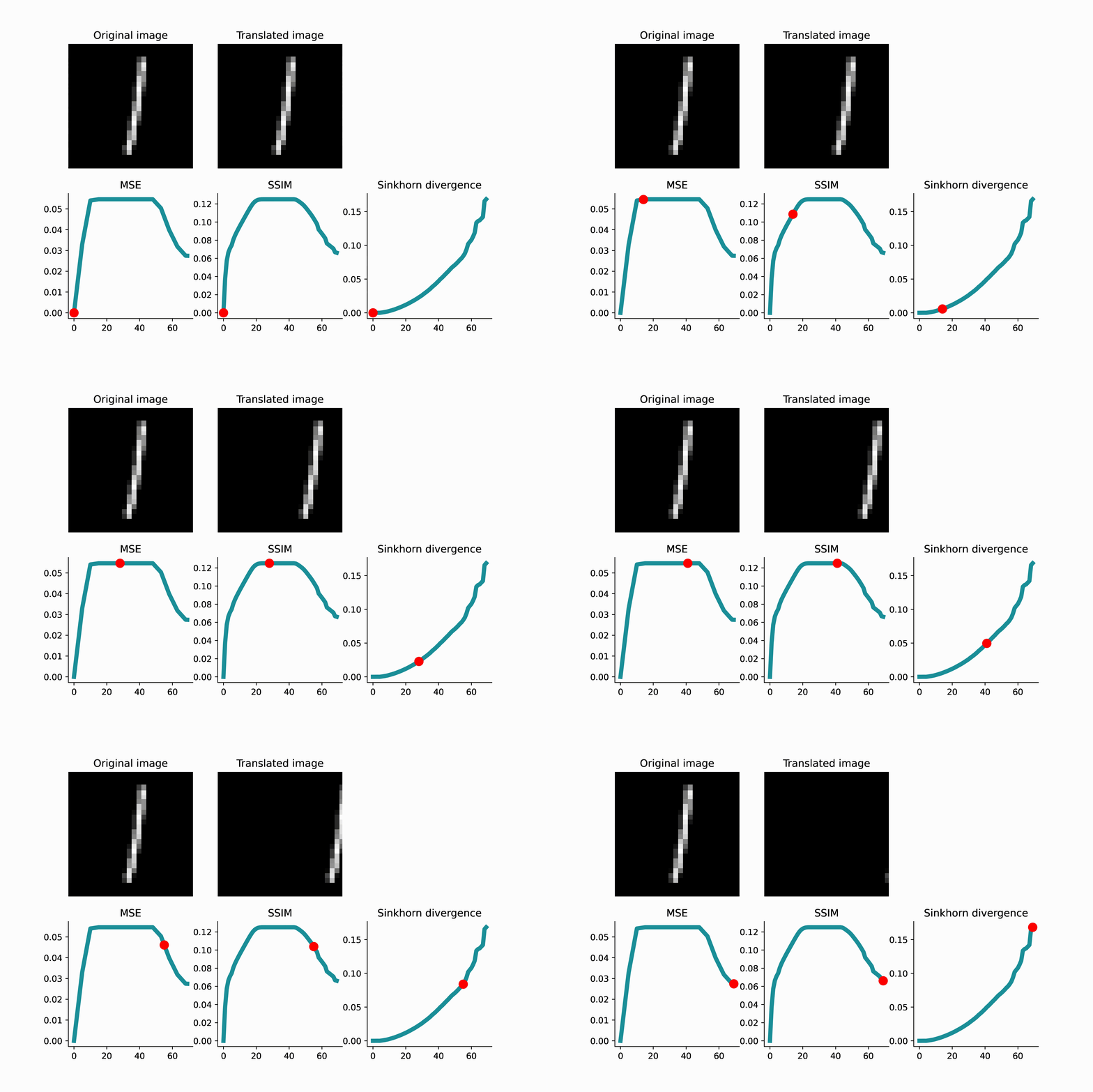
To visually see that MSE is not a reliable indicator of translation distance, see the GIFs presented below. As a first example, an MNIST image of ‘1’ is translated, and when the translated image and the original image do not overlap, the MSE remains constant. This can lead to complications if one uses gradient-based optimization to minimize the loss.

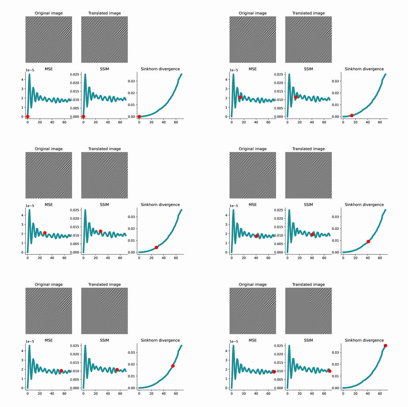
As another example below, an image of high-frequency textures (a curvelet band of an image) is translated. Since the curvelet is oscillatory, the MSE loss has many local minima. Again, this can make gradient-based optimization difficult.

As we see in the above GIFS, the Sinkhorn divergence produces a smooth and monotonic curve, which agrees with our intuition of translation distance.

The Google Colab notebook for reproducing these experiments can be found here.